Process
i
OPTION 1:
OPTION 2:
View Lab Activity as it unfolds in the webpage area below:
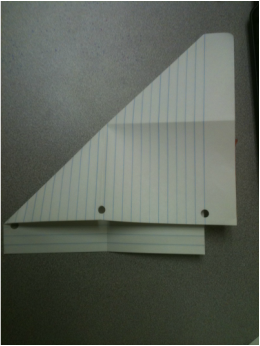
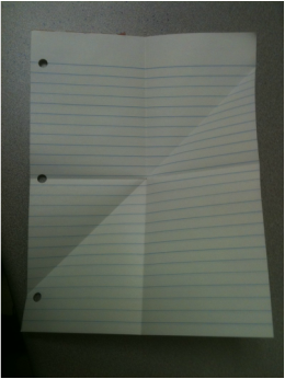
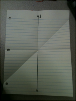
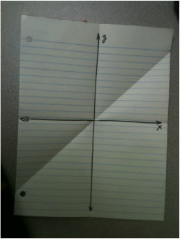
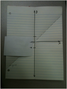
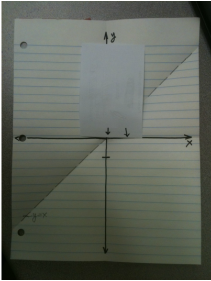
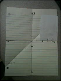
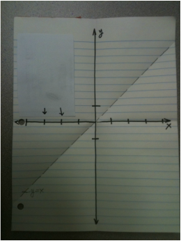
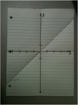
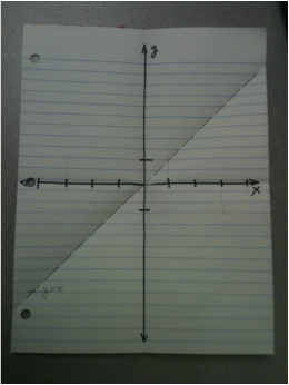
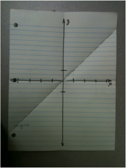
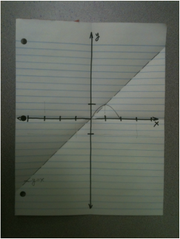
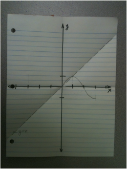
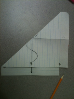
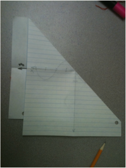
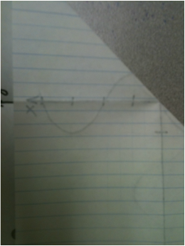
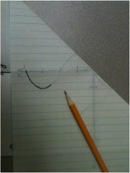
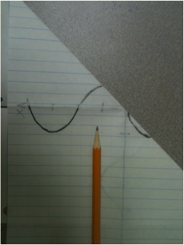
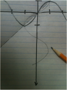
There are many steps... so read each instruction carefully and look at the accompanying photographs carefully for additional insight.
There are many steps... so read each instruction carefully and look at the accompanying photographs carefully for additional insight.
|
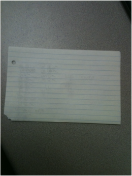
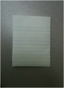
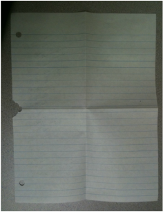
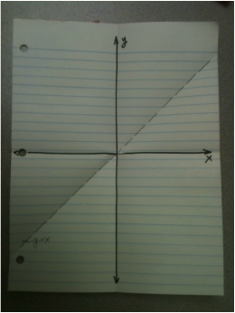
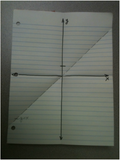
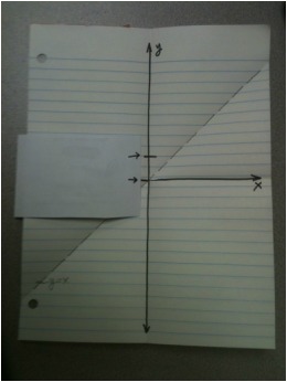
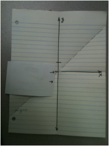
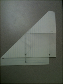
Carefully tear out a single piece of standard notebook paper. |

|
|
|
|
|
|
|
|
|
|
|
|
|
|
|
|
|
|
|
|
|
|
|
|
|
|
|
|
|
|
|
|
|
|
|
|
|
|
|
|
|
|
|
|
|
|
|
|
|
|
|
|
|
|
|
|
|
|
|
|
|
|
|
|
|
|
|
|
|
|
|
|
|
|
|
|
|
|
|
|
Good luck and begin...
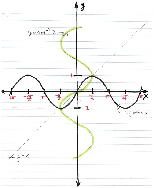
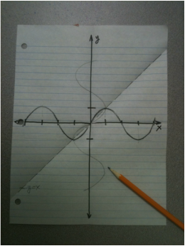
Exemplar: